PyTorch Geometric

PyTorch Geometric (PyG) は、幾何学的ディープラーニングにおいて最も人気のあるライブラリの 1 つです。W&B は PyG と非常に相性が良く、グラフの可視化や Experiments の追跡をスムーズに行うことができます。

PyTorch Geometric をインストールした後、以下の手順に従って開始してください。

​

サインアップと APIキー の作成

APIキー は、お使いのマシンを W&B に対して認証するために使用されます。 APIキー はユーザープロフィールから生成できます。

For a more streamlined approach, create an API key by going directly to User Settings. Copy the newly created API key immediately and save it in a secure location such as a password manager.

1. 右上隅にあるユーザープロフィールのアイコンをクリックします。
2. User Settings を選択し、 API Keys セクションまでスクロールします。

​

wandb ライブラリのインストールとログイン

ローカル環境に wandb ライブラリをインストールしてログインするには：

Command Line

1. WANDB_API_KEY 環境変数 に作成した APIキー を設定します。

   export WANDB_API_KEY=<your_api_key>
   

2. wandb ライブラリをインストールしてログインします。

   pip install wandb
   
   wandb login
   

Python

pip install wandb

import wandb
wandb.login()

Python notebook

!pip install wandb

import wandb
wandb.login()

​

グラフの可視化

エッジの数やノードの数など、入力グラフの詳細を保存できます。W&B は Plotly チャートや HTML パネルのログ記録をサポートしているため、グラフ用に作成したあらゆる可視化を W&B にログとして記録できます。

​

PyVis の使用

以下のスニペットは、PyVis と HTML を使用して可視化を行う方法を示しています。

from pyvis.network import Network
import wandb

# 'graph_vis' というプロジェクトで run を初期化
with wandb.init(project=’graph_vis’) as run:
    net = Network(height="750px", width="100%", bgcolor="#222222", font_color="white")

    # PyG グラフから PyVis ネットワークにエッジを追加
    for e in tqdm(g.edge_index.T):
        src = e[0].item()
        dst = e[1].item()

        net.add_node(dst)
        net.add_node(src)
        
        net.add_edge(src, dst, value=0.1)

    # PyVis の可視化を HTML ファイルとして保存
    net.show("graph.html")
    # HTML ファイルを W&B にログ記録
    run.log({"eda/graph": wandb.Html("graph.html")})

​

Plotly の使用

Plotly を使用してグラフの可視化を作成するには、まず PyG グラフを networkx オブジェクトに変換する必要があります。その後、ノードとエッジの両方に対して Plotly の scatter plot を作成します。以下のスニペットをこのタスクに使用できます。

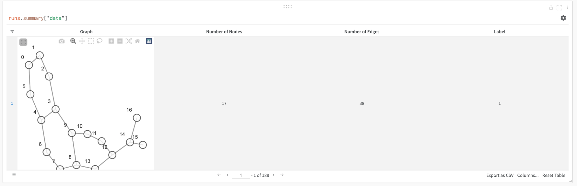
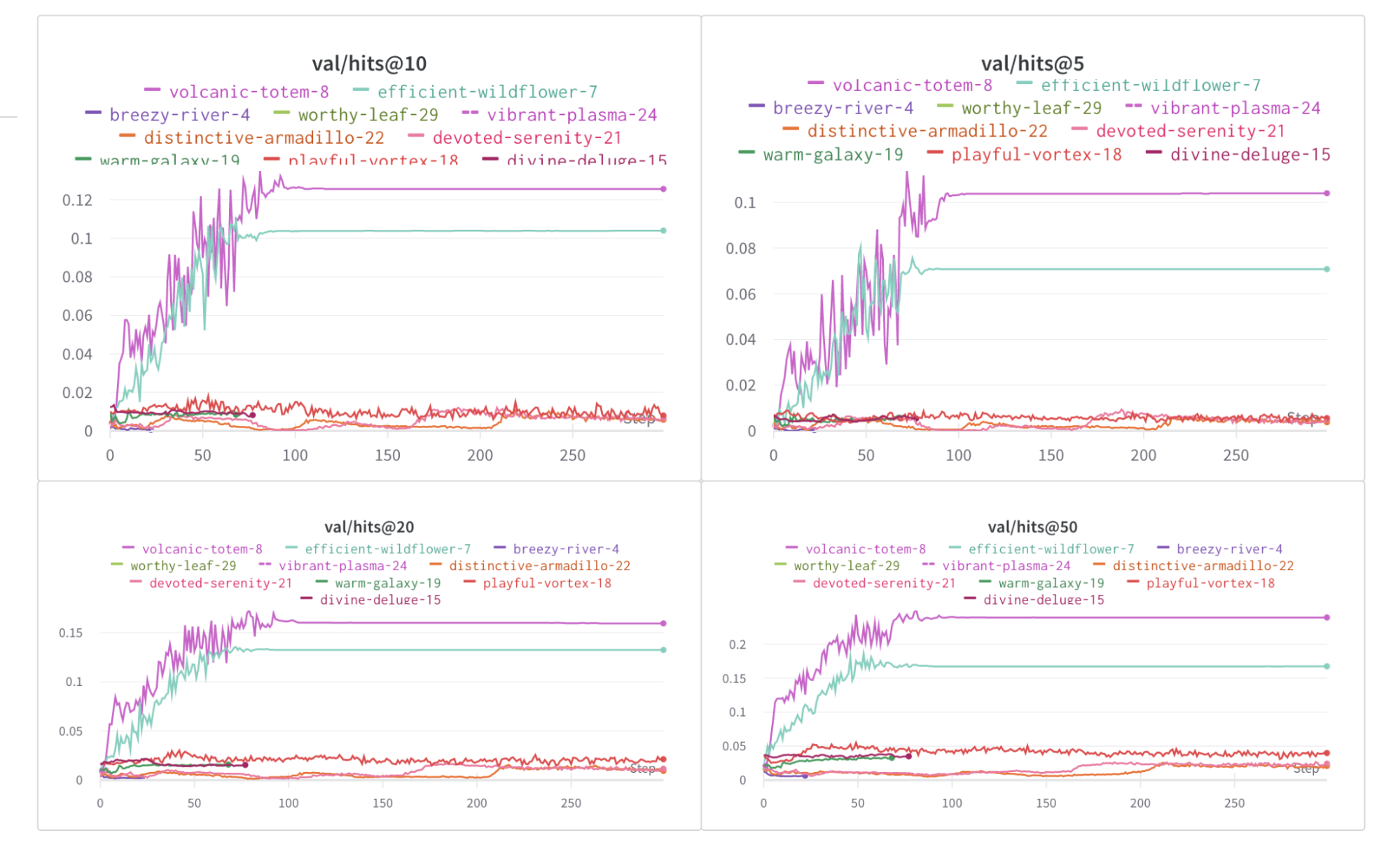
def create_vis(graph):
    G = to_networkx(graph)
    pos = nx.spring_layout(G)

    edge_x = []
    edge_y = []
    for edge in G.edges():
        x0, y0 = pos[edge[0]]
        x1, y1 = pos[edge[1]]
        edge_x.append(x0)
        edge_x.append(x1)
        edge_x.append(None)
        edge_y.append(y0)
        edge_y.append(y1)
        edge_y.append(None)

    edge_trace = go.Scatter(
        x=edge_x, y=edge_y,
        line=dict(width=0.5, color='#888'),
        hoverinfo='none',
        mode='lines'
    )

    node_x = []
    node_y = []
    for node in G.nodes():
        x, y = pos[node]
        node_x.append(x)
        node_y.append(y)

    node_trace = go.Scatter(
        x=node_x, y=node_y,
        mode='markers',
        hoverinfo='text',
        line_width=2
    )

    fig = go.Figure(data=[edge_trace, node_trace], layout=go.Layout())

    return fig


with wandb.init(project=’visualize_graph’) as run:
    # Plotly オブジェクトを W&B にログ記録
    run.log({‘graph’: wandb.Plotly(create_vis(graph))})

​

メトリクスのログ記録

W&B を使用して、損失関数（loss）や精度（accuracy）などの実験と関連メトリクスを追跡できます。トレーニングループに以下の行を追加してください。

with wandb.init(project="my_project", entity="my_entity") as run:
    # メトリクスを W&B にログ記録
    run.log({
        'train/loss': training_loss,
        'train/acc': training_acc,
        'val/loss': validation_loss,
        'val/acc': validation_acc
        })

​

その他のリソース

• Recommending Amazon Products using Graph Neural Networks in PyTorch Geometric
• Point Cloud Classification using PyTorch Geometric
• Point Cloud Segmentation using PyTorch Geometric